The functional component of AFM scanners is typically piezoelectric material such as PZT (lead zirconium titanate). Piezo materials contract and elongate when voltage is applied, according to whether the voltage is negative or positive, and depending upon the orientation of the material’s polarized grain structure. Piezoelectric Scanners are used to precisely manipulate sample-tip movement in order to scan the sample surface. In Dimension SPMs, the sample is stationary while the scanner moves the tip (this is true for both Dimension Icon and Dimension FastScan scanners).
Not all scanners react exactly the same to a given voltage. Because of slight variations in the orientation and size of the piezoelectric granular structure (polarity), material thickness, etc., each scanner has a unique “personality.” This personality is conveniently measured in terms of sensitivity: the ratio of piezo movement to piezo voltage. Sensitivity is not a linear relationship, however. Because piezo scanners exhibit more sensitivity (i.e., more movement per volt) at higher voltages than they do at lower voltages, the sensitivity curve is just that—curved. This non-linear relationship is determined for each scanner crystal and follows it for the life of the scanner. As the scanner ages, its sensitivity will decrease somewhat, necessitating periodic recalibration.
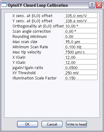
The Calibrate > Scanner > XY... function displays the OptoXY Closed Loop Calibration dialog box, allowing users to enter the sensitivity of their scanner’s XY axes.
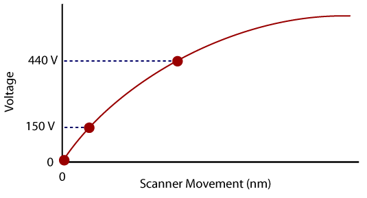
Sensitivity is measured in terms of lateral displacement for a given voltage (nm/V). The NanoScope software employs various derating and coupling parameters to model scanners’ nonlinear characteristics. By precisely determining points along the scanner’s sensitivity curve, then applying a rigorous mathematical model, full-range measuring capabilities can be achieved with better than 1% accuracy. Consider the sensitivity curve below:
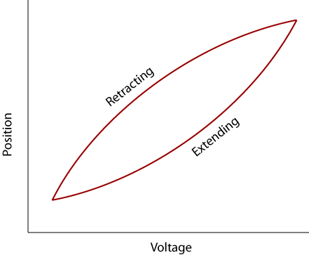
However, because piezo materials exhibit hysteresis, their response to increasing voltage is not the same as their response to decreasing voltage. That is, piezo materials exhibit “memory”, which causes the scanner to behave differently as voltages recede toward zero. The graph below represents this relationship:
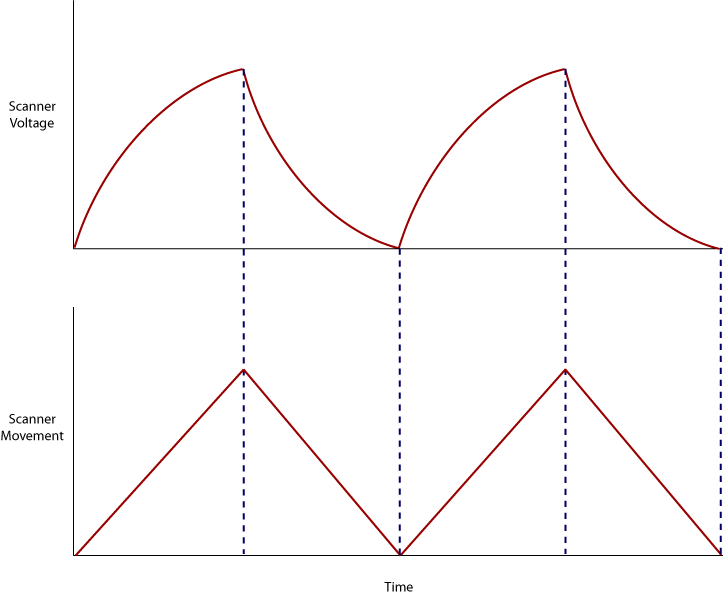
To produce the sharp, linear movements (triangular waveform) required for accurate raster scanning, it is necessary to shape the applied voltage as shown below:
In addition to nonlinearity and hysteresis, the applied voltage must compensate for scan rate and scan size. As scan rate slows, the applied voltage must compensate for increased memory effects in the piezo material. As scan size is decreased, the piezo exhibits more linearity. These effects are further complicated by X-Y-Z coupling effects (the tendency for one axis to affect movement in other axes).
Through rigorous quality control of its scanner piezos, Bruker has achieved excellent modeling of scanner characteristics. Two calibration points are typically used for fine-tuning: 150 and 440 V. A third point is assumed at 0 V. These three points yield a second-order sensitivity curve to ensure accurate measurements throughout a broad range of scanner movements.
Because scanner sensitivities vary according to how much voltage is applied to them, the reference must be thoroughly scanned at a variety of sizes and angles. The user dictates, via the software, the distance between known features on the reference’s surface and a parameter is recorded to compensate for the scanner’s characteristics. The X, Y and Z axes may be calibrated in any sequential order; however, Linearity Correction must be performed before any calibrations are attempted. Otherwise, calibrations will be undone by the linearity adjustments.
| www.bruker.com | Bruker Corporation |
| www.brukerafmprobes.com | 112 Robin Hill Rd. |
| nanoscaleworld.bruker-axs.com/nanoscaleworld/ | Santa Barbara, CA 93117 |
| Customer Support: (800) 873-9750 | |
| Copyright 2010, 2011. All Rights Reserved. |